GPU-accelerated climate modeling
Climate modeling is hard for two reasons: data and compute. Satellite imagery arrives continuously from multiple sources. Reanalysis datasets have to be pulled from remote APIs. Weather station data shows up in different formats and schemas. And once all of that is finally in one place, running atmospheric physics simulations demands serious GPU compute.
In practice, many climate workflows are held together with scripts, cron jobs, and a lot of manual babysitting. Data ingestion breaks without warning. GPU jobs run overnight with little visibility into what’s happening. When something interesting shows up in a simulation, like a developing hurricane, no one notices until the job finishes hours later.
In this tutorial, we build a production-grade climate modeling pipeline using Flyte. We ingest data from three different sources in parallel, combine it with Dask, run ensemble atmospheric simulations on H200 GPUs, detect extreme weather events as they emerge, and visualize everything in a live dashboard. The entire pipeline is orchestrated, cached, and fault-tolerant, so it can run reliably at scale.
Full code available here.
Overview
We’re building an ensemble weather forecasting system. Ensemble forecasting runs the same simulation multiple times with slightly different initial conditions. This quantifies forecast uncertainty. Instead of saying “the temperature will be 25°C”, we can say “the temperature will be 24-26°C with 90% confidence”.
The pipeline has five stages:
- Data ingestion: Pull satellite imagery from NOAA GOES, reanalysis data from ERA5, and surface observations from weather stations in parallel.
- Preprocessing: Fuse the datasets, interpolate to a common grid, and run quality control using Dask for distributed computation.
- GPU simulation: Run ensemble atmospheric physics on H200 GPUs. Each ensemble member evolves independently. PyTorch handles the tensor operations;
torch.compileoptimizes the kernels. - Event detection: Monitor for hurricanes (high wind + low pressure) and heatwaves during simulation. When extreme events are detected, the pipeline can adaptively refine the grid resolution.
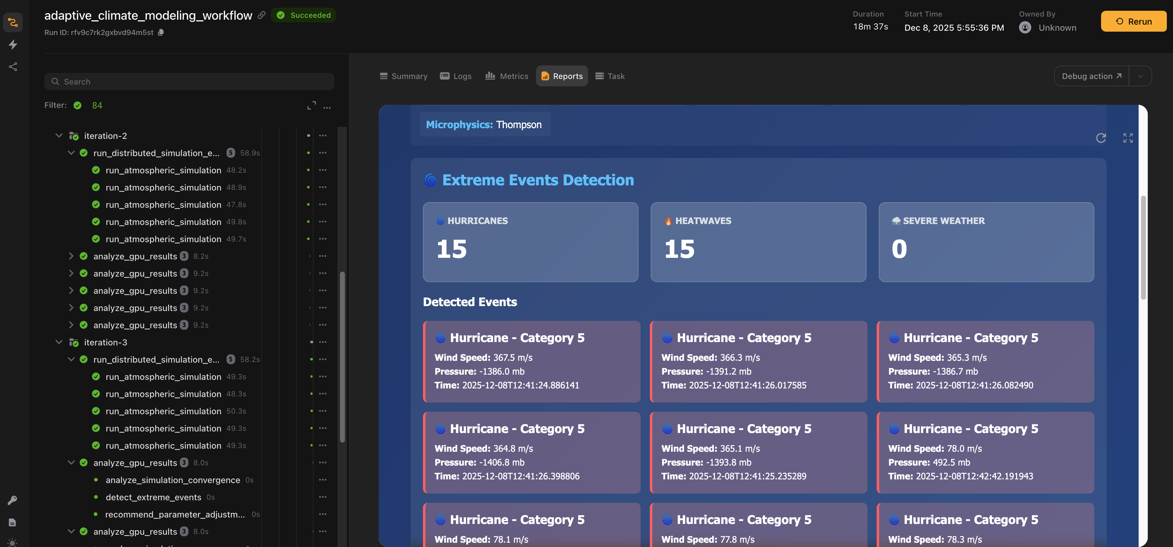
- Real-time reporting: Stream metrics to a live Flyte Reports dashboard showing convergence and detected events.
This workflow is a good example of where Flyte shines!
- Parallel data ingestion: Three different data sources, three different APIs, all running concurrently. Flyte’s async task execution handles this naturally.
- Resource heterogeneity: Data ingestion needs CPU and network. Preprocessing needs a Dask cluster. Simulation needs GPUs. Flyte provisions exactly what each stage needs.
- Caching: ERA5 data fetches can take minutes. Run the pipeline twice with the same date range, and Flyte skips the fetch entirely.
- Adaptive workflows: When a hurricane is detected, we can dynamically refine the simulation. Flyte makes this kind of conditional logic straightforward.
Implementation
Dependencies and container image
import asyncio
import gc
import io
import json
import os
import tempfile
from dataclasses import dataclass
from datetime import datetime, timedelta
from typing import Literal

import flyte
import numpy as np
import pandas as pd
import xarray as xr
from flyte.io import File
from flyteplugins.dask import Dask, Scheduler, WorkerGroup
The key imports include xarray for multi-dimensional climate data, flyteplugins.dask for distributed preprocessing, and flyte for orchestration.
climate_image = (
    flyte.Image.from_debian_base(name="climate_modeling_h200")
    .with_apt_packages(
        "libnetcdf-dev",  # NetCDF for climate data
        "libhdf5-dev",  # HDF5 for large datasets
        "libeccodes-dev",  # GRIB format support (ECMWF's native format)
        "libudunits2-dev",  # Unit conversions
    )
    .with_pip_packages(
        "numpy==2.3.5",
        "pandas==2.3.3",
        "xarray==2025.11.0",
        "torch==2.9.1",
        "netCDF4==1.7.3",
        "s3fs==2025.10.0",
        "aiohttp==3.13.2",
        "ecmwf-datastores-client==0.4.1",
        "h5netcdf==1.7.3",
        "cfgrib==0.9.15.1",
        "pyarrow==22.0.0",
        "scipy==1.15.1",
        "flyteplugins-dask>=2.0.0b33",
        "nvidia-ml-py3==7.352.0",
    )
    .with_env_vars({"PYTORCH_CUDA_ALLOC_CONF": "max_split_size_mb:512"})
)
Climate data comes in specialized formats such as NetCDF, HDF5, and GRIB. The container image includes libraries to work with all of them, along with PyTorch for GPU computation and the ECMWF client for accessing ERA5 data.
Simulation parameters and data structures
@dataclass
class SimulationParams:
    grid_resolution_km: float = 10.0
    time_step_minutes: int = 10
    simulation_hours: int = 240
    physics_model: Literal["WRF", "MPAS", "CAM"] = "WRF"
    boundary_layer_scheme: str = "YSU"
    microphysics_scheme: str = "Thompson"
    radiation_scheme: str = "RRTMG"

    # Ensemble forecasting parameters
    ensemble_size: int = 800
    perturbation_magnitude: float = 0.5

    # Convergence criteria for adaptive refinement
    convergence_threshold: float = 0.1  # 10% of initial ensemble spread
    max_iterations: int = 3


@dataclass
class ClimateMetrics:
    timestamp: str
    iteration: int
    convergence_rate: float
    energy_conservation_error: float
    max_wind_speed_mps: float
    min_pressure_mb: float
    detected_phenomena: list[str]
    compute_time_seconds: float
    ensemble_spread: float


@dataclass
class SimulationSummary:
    total_iterations: int
    final_resolution_km: float
    avg_convergence_rate: float
    total_compute_time_seconds: float
    hurricanes_detected: int
    heatwaves_detected: int
    converged: bool
    region: str
    output_files: list[File]
    date_range: list[str, str]
SimulationParams defines the core behavior of the simulation, including grid resolution, physics schemes, and ensemble size. The default configuration runs 800 ensemble members, which is sufficient to produce statistically meaningful uncertainty estimates.
Decreasing the grid spacing via grid_resolution_km (for example, from 10 km to 5 km) increases grid resolution and significantly increases memory usage because it introduces more data points and intermediate state. Even with 141 GB of H200 GPU memory, high-resolution or adaptively refined simulations may exceed available VRAM, especially when running large ensembles.
To mitigate this, consider reducing the ensemble size, limiting the refined region, running fewer physics variables, or scaling the simulation across more GPUs so memory is distributed more evenly.
ClimateMetrics collects diagnostics at each iteration, such as convergence rate, energy conservation, and detected phenomena. These metrics are streamed to the real-time dashboard so you can monitor how the simulation evolves as it runs.
Task environments
Different stages need different resources. Flyte’s TaskEnvironment declares exactly what each task requires:
gpu_env = flyte.TaskEnvironment(
    name="climate_modeling_gpu",
    resources=flyte.Resources(
        cpu=5,
        memory="130Gi",
        gpu="H200:1",
    ),
    image=climate_image,
    cache="auto",
)

dask_env = flyte.TaskEnvironment(
    name="climate_modeling_dask",
    plugin_config=Dask(
        scheduler=Scheduler(resources=flyte.Resources(cpu=2, memory="6Gi")),
        workers=WorkerGroup(
            number_of_workers=2,
            resources=flyte.Resources(cpu=2, memory="12Gi"),
        ),
    ),
    image=climate_image,
    resources=flyte.Resources(cpu=2, memory="12Gi"),  # Head node
    cache="auto",
)


cpu_env = flyte.TaskEnvironment(
    name="climate_modeling_cpu",
    resources=flyte.Resources(cpu=8, memory="64Gi"),
    image=climate_image,
    cache="auto",
    secrets=[
        flyte.Secret(key="cds_api_key", as_env_var="ECMWF_DATASTORES_KEY"),
        flyte.Secret(key="cds_api_url", as_env_var="ECMWF_DATASTORES_URL"),
    ],
    depends_on=[gpu_env, dask_env],
)
Here’s what each environment is responsible for:
gpu_env: Runs the atmospheric simulations on H200 GPUs. The 130 GB of GPU memory is used to hold the ensemble members in VRAM during execution.dask_env: Provides a distributed Dask cluster for preprocessing. A scheduler and multiple workers handle data fusion and transformation in parallel.cpu_env: Handles data ingestion and orchestration. This environment also includes the secrets required to access the ERA5 API.
The depends_on setting on cpu_env ensures that Flyte builds the GPU and Dask images first. Once those environments are ready, the orchestration task can launch the specialized simulation and preprocessing tasks.
Data ingestion: multiple sources in parallel
Climate models need data from multiple sources. Each source has different formats, APIs, and failure modes. We handle them as separate Flyte tasks that run concurrently.
Satellite imagery from NOAA GOES
@cpu_env.task
async def ingest_satellite_data(region: str, date_range: list[str, str]) -> File:
    """Ingest GOES satellite imagery from NOAA's public S3 buckets."""
This task fetches cloud imagery and precipitable water products from NOAA’s public S3 buckets. GOES-16 covers the Atlantic; GOES-17 covers the Pacific. The task selects the appropriate satellite based on region, fetches multiple days in parallel using asyncio.gather, and combines everything into a single xarray Dataset.
ERA5 reanalysis from Copernicus
@cpu_env.task
async def ingest_reanalysis_data(region: str, date_range: list[str, str]) -> File:
    """Fetch ERA5 reanalysis from Copernicus Climate Data Store."""
ERA5 provides 3D atmospheric fields such as temperature, wind, humidity at multiple pressure levels from surface to stratosphere. The ECMWF datastores client handles authentication via Flyte secrets. Each day fetches in parallel, then gets concatenated.
Surface observations from weather stations:
@cpu_env.task
async def ingest_station_data(
    region: str, date_range: list[str, str], max_stations: int = 100
) -> File:
    """Fetch ground observations from NOAA's Integrated Surface Database."""
Ground truth comes from NOAA’s Integrated Surface Database. The task filters stations by geographic bounds, fetches hourly observations, and returns a Parquet file for efficient downstream processing.
All three tasks return Flyte File objects that hold references to data in blob storage. No data moves until a downstream task actually needs it.
Preprocessing with Dask
The three data sources need to be combined into a unified atmospheric state. This means:
- Interpolating to a common grid
- Handling missing values
- Merging variables from different sources
- Quality control
This is a perfect fit for Dask to handle lazy evaluation over chunked arrays:
@dask_env.task
async def preprocess_atmospheric_data(
    satellite_data: File,
    reanalysis_data: File,
    station_data: File,
    target_resolution_km: float,
) -> File:
This task connects to the Dask cluster provisioned by Flyte, loads the datasets with appropriate chunking, merges satellite and reanalysis grids, fills in missing values, and persists the result. Flyte caches the output, so preprocessing only runs when the inputs change.
GPU-accelerated atmospheric simulation
Now the core: running atmospheric physics on the GPU. Each ensemble member is an independent forecast with slightly perturbed initial conditions.
@gpu_env.task
async def run_atmospheric_simulation(
    input_data: File,
    params: SimulationParams,
    partition_id: int = 0,
    ensemble_start: int | None = None,
    ensemble_end: int | None = None,
) -> tuple[File, ClimateMetrics]:
    """Run GPU-accelerated atmospheric simulation with ensemble forecasting."""
The task accepts a subset of ensemble members (ensemble_start to ensemble_end). This enables distributing 800 members across multiple GPUs.
The physics step is the computational kernel. It runs advection (wind transport), pressure gradients, Coriolis forces, turbulent diffusion, and moisture condensation:
    @torch.compile(mode="reduce-overhead")
    def physics_step(state_tensor, dt_val, dx_val):
        """Compiled atmospheric physics - 3-4x faster with torch.compile."""
        # Advection: transport by wind
        temp_grad_x = torch.roll(state_tensor[:, 0], -1, dims=2) - torch.roll(
            state_tensor[:, 0], 1, dims=2
        )
        temp_grad_y = torch.roll(state_tensor[:, 0], -1, dims=3) - torch.roll(
            state_tensor[:, 0], 1, dims=3
        )
        advection = -(
            state_tensor[:, 3] * temp_grad_x + state_tensor[:, 4] * temp_grad_y
        ) / (2 * dx_val)
        state_tensor[:, 0] = state_tensor[:, 0] + advection * dt_val

        # Pressure gradient with Coriolis
        pressure_grad_x = (
            torch.roll(state_tensor[:, 1], -1, dims=2)
            - torch.roll(state_tensor[:, 1], 1, dims=2)
        ) / (2 * dx_val)
        pressure_grad_y = (
            torch.roll(state_tensor[:, 1], -1, dims=3)
            - torch.roll(state_tensor[:, 1], 1, dims=3)
        ) / (2 * dx_val)

        coriolis_param = 1e-4  # ~45°N latitude
        coriolis_u = coriolis_param * state_tensor[:, 4]
        coriolis_v = -coriolis_param * state_tensor[:, 3]

        state_tensor[:, 3] = (
            state_tensor[:, 3] - pressure_grad_x * dt_val * 0.01 + coriolis_u * dt_val
        )
        state_tensor[:, 4] = (
            state_tensor[:, 4] - pressure_grad_y * dt_val * 0.01 + coriolis_v * dt_val
        )

        # Turbulent diffusion
        diffusion_coeff = 10.0
        laplacian_temp = (
            torch.roll(state_tensor[:, 0], 1, dims=2)
            + torch.roll(state_tensor[:, 0], -1, dims=2)
            + torch.roll(state_tensor[:, 0], 1, dims=3)
            + torch.roll(state_tensor[:, 0], -1, dims=3)
            - 4 * state_tensor[:, 0]
        ) / (dx_val * dx_val)
        state_tensor[:, 0] = (
            state_tensor[:, 0] + diffusion_coeff * laplacian_temp * dt_val
        )

        # Moisture condensation
        sat_vapor_pressure = 611.2 * torch.exp(
            17.67 * state_tensor[:, 0] / (state_tensor[:, 0] + 243.5)
        )
        condensation = torch.clamp(
            state_tensor[:, 2] - sat_vapor_pressure * 0.001, min=0
        )
        state_tensor[:, 2] = state_tensor[:, 2] - condensation * 0.1
        state_tensor[:, 0] = state_tensor[:, 0] + condensation * 2.5e6 / 1005 * dt_val

        return state_tensor
@torch.compile(mode="reduce-overhead") compiles this function into optimized CUDA kernels. Combined with mixed precision (torch.cuda.amp.autocast), this runs 3-4x faster than eager PyTorch.
Every 10 timesteps, the simulation checks for extreme events:
- Hurricanes: Wind speed > 33 m/s with low pressure
- Heatwaves: Temperature anomalies exceeding thresholds
Detected phenomena get logged to the metrics, which flow to the live dashboard.
Distributing across multiple GPUs
800 ensemble members is a lot for one GPU, so we distribute them:
@cpu_env.task
async def run_distributed_simulation_ensemble(
    preprocessed_data: File, params: SimulationParams, n_gpus: int
) -> tuple[list[File], list[ClimateMetrics]]:
    total_members = params.ensemble_size
    members_per_gpu = total_members // n_gpus

    # Distribute ensemble members across GPUs
    tasks = []
    for gpu_id in range(n_gpus):
        # Calculate ensemble range for this GPU
        ensemble_start = gpu_id * members_per_gpu
        # Last GPU gets any remainder members
        if gpu_id == n_gpus - 1:
            ensemble_end = total_members
        else:
            ensemble_end = ensemble_start + members_per_gpu

        # Launch GPU task with ensemble subset
        gpu_task = run_atmospheric_simulation(
            preprocessed_data,
            params,
            gpu_id,
            ensemble_start=ensemble_start,
            ensemble_end=ensemble_end,
        )
        tasks.append(gpu_task)

    # Execute all GPUs in parallel
    results = await asyncio.gather(*tasks)

    output_files = [r[0] for r in results]
    metrics = [r[1] for r in results]

    return output_files, metrics
The task splits the ensemble members evenly across the available GPUs, launches the simulation runs in parallel using asyncio.gather, and then aggregates the results. With five GPUs, each GPU runs 160 ensemble members. Flyte takes care of scheduling, so GPU tasks start automatically as soon as resources become available.
The main workflow
Everything comes together in the orchestration task:
@cpu_env.task(report=True)
async def adaptive_climate_modeling_workflow(
    region: str = "atlantic",
    date_range: list[str, str] = ["2024-09-01", "2024-09-10"],
    current_params: SimulationParams = SimulationParams(),
    enable_multi_gpu: bool = True,
    n_gpus: int = 5,
) -> SimulationSummary:
    """Orchestrates multi-source ingestion, GPU simulation, and adaptive refinement."""
report=True enables Flyte Reports for live monitoring.
    # Parallel data ingestion from three sources
    with flyte.group("data-ingestion"):
        satellite_task = ingest_satellite_data(region, date_range)
        reanalysis_task = ingest_reanalysis_data(region, date_range)
        station_task = ingest_station_data(region, date_range)

        satellite_data, reanalysis_data, station_data = await asyncio.gather(
            satellite_task,
            reanalysis_task,
            station_task,
        )
flyte.group("data-ingestion") visually groups the ingestion tasks in the Flyte UI. Inside the group, three tasks launch concurrently. asyncio.gather waits for all three to complete before preprocessing begins.
The workflow then enters an iterative loop:
- Run GPU simulation (single or multi-GPU)
- Check convergence by comparing forecasts across iterations
- Detect extreme events
- If a hurricane is detected and we haven’t refined yet, double the grid resolution
- Stream metrics to the live dashboard
- Repeat until converged or max iterations reached
Adaptive mesh refinement is the key feature here. When the simulation detects a hurricane forming, it automatically increases resolution to capture the fine-scale dynamics. This is expensive, so we limit it to one refinement per run.
Running the pipeline
if __name__ == "__main__":
    flyte.init_from_config()
    run_multi_gpu = flyte.run(adaptive_climate_modeling_workflow)

    print(f"Run URL: {run_multi_gpu.url}")
Before running, set up ERA5 API credentials:
flyte create secret cds_api_key <YOUR_CDS_API_KEY>
flyte create secret cds_api_url https://cds.climate.copernicus.eu/api
Then launch:
flyte create config --endpoint <FLYTE_OR_UNION_ENDPOINT> --project <PROJECT_NAME> --domain <DOMAIN_NAME> --builder remote
uv run simulation.py
The default configuration uses the Atlantic region for September 2024, which is hurricane season.
Key concepts
Ensemble forecasting
Weather prediction is inherently uncertain. Small errors in the initial conditions grow over time due to chaotic dynamics, which means a single forecast can only ever be one possible outcome.
Ensemble forecasting addresses this uncertainty by:
- Perturbing the initial conditions within known observational error bounds
- Running many independent forecasts
- Computing the ensemble mean as the most likely outcome and the ensemble spread as a measure of uncertainty
Adaptive mesh refinement
When a hurricane begins to form, coarse spatial grids are not sufficient to resolve critical features like eyewall dynamics. Adaptive mesh refinement allows the simulation to focus compute where it matters most by:
- Increasing grid resolution, for example from 10 km to 5 km
- Reducing the timestep to maintain numerical stability
- Refining only the regions of interest instead of the entire domain
This approach is computationally expensive, but it is essential for producing accurate intensity forecasts.
Real-time event detection
Rather than analyzing results after a simulation completes, this pipeline detects significant events as the simulation runs.
The system monitors for conditions such as:
- Hurricanes: Wind speeds exceeding 33 m/s (Category 1 threshold) combined with central pressure below 980 mb
- Heatwaves: Sustained temperature anomalies over a defined period
Detecting these events in real time enables adaptive responses, such as refining the simulation or triggering alerts, and supports earlier warnings for extreme weather.
Where to go next
This example is intentionally scoped to keep the ideas clear, but there are several natural ways to extend it for more realistic workloads.
To model different ocean basins, change the region parameter to values like "pacific" or "indian". The ingestion tasks automatically adjust to pull the appropriate satellite coverage for each region.
To run longer forecasts, increase simulation_hours in SimulationParams. The default of 240 hours, or 10 days, is typical for medium-range forecasting, but you can run longer simulations if you have the compute budget.
Finally, the physics step here is deliberately simplified. Production systems usually incorporate additional components such as radiation schemes, boundary layer parameterizations, and land surface models. These can be added incrementally as separate steps without changing the overall structure of the pipeline.