Distributed LLM pretraining
When training large models, infrastructure should not be the hardest part. The real work is in the model architecture, the data, and the hyperparameters. In practice, though, teams often spend weeks just trying to get distributed training to run reliably.
And when it breaks, it usually breaks in familiar ways: out-of-memory crashes, corrupted checkpoints, data loaders that silently fail, or runs that hang with no obvious explanation.
Most distributed training tutorials focus on PyTorch primitives. This one focuses on getting something that actually ships. We go into the technical details, such as how FSDP shards parameters, why gradient clipping behaves differently at scale, and how streaming datasets reduce memory pressure, but always with the goal of building a system that works in production.
Real training jobs need more than a training loop. They need checkpointing, fault tolerance, data streaming, visibility into what’s happening, and the ability to recover from failures. In this tutorial, we build all of that using Flyte, without having to stand up or manage any additional infrastructure.
Full code available here.
Overview
We’re going to pretrain a GPT-2 style language model from scratch. This involves training on raw text data starting from randomly initialized weights, rather than fine-tuning or adapting a pretrained model. This is the same process used to train the original GPT-2, LLaMA, and most other foundation models.
The model learns by predicting the next token. Given “The cat sat on the”, it learns to predict “mat”. Do this billions of times across terabytes of text, and the model develops surprisingly sophisticated language understanding. That’s pretraining.
The challenge is scale. A 30B parameter model doesn’t fit on a single GPU. The training dataset, SlimPajama in our case, is 627 billion tokens. Training runs last for days or even weeks. To make this work, you need:
- Distributed training: Split the model across multiple GPUs using FSDP (Fully Sharded Data Parallel)
- Data streaming: Pull training data on-demand instead of downloading terabytes upfront
- Checkpointing: Save progress regularly so a failure doesn’t wipe out days of compute
- Observability: See what’s happening inside a multi-day training run
We’ll build a Flyte pipeline that takes care of all of this, using three tasks with clearly defined responsibilities:
- Data preparation: Tokenizes your dataset and converts it to MDS (MosaicML Data Shard) format for streaming. This Flyte task is cached, so it only needs to be run once and can be reused across runs.
- Distributed training: Runs FSDP across 8 H200 GPUs. Flyte’s
Elasticplugin handles the distributed setup. Checkpoints upload to S3 automatically via Flyte’sFileabstraction. - Real-time reporting: Streams loss curves and training metrics to Flyte Reports, a live dashboard integrated into the Flyte UI.
Why three separate tasks? Flyte makes this separation efficient:
- Caching: The data preparation step runs once. On subsequent runs, Flyte skips it entirely.
- Resource isolation: Training uses expensive H200 GPUs only while actively training, while the driver runs on inexpensive CPU instances.
- Fault boundaries: If training fails, the data preparation step does not re-run. Training can resume directly from the most recent checkpoint.
Implementation
Let’s walk through the code. We’ll start with the infrastructure setup, build the model, then wire everything together into a pipeline.
Setting up the environment
Every distributed training job needs a consistent environment across all nodes. Flyte handles this with container images:
import logging
import math
import os
from pathlib import Path
from typing import Optional

import flyte
import flyte.report
import lightning as L
import numpy as np
import torch
import torch.nn as nn
from flyte.io import Dir, File
from flyteplugins.pytorch.task import Elastic
The imports tell the story: flyte for orchestration, flyte.report for live dashboards, lightning for training loop management, and Elastic from Flyte’s PyTorch plugin. This last one is key as it configures PyTorch’s distributed launch without you writing any distributed setup code.
NUM_NODES = 1
DEVICES_PER_NODE = 8
VOCAB_SIZE = (
    50257  # GPT-2 BPE tokenizer vocabulary size (constant across all model sizes)
)
N_POSITIONS = 2048  # Maximum sequence length (constant across all model sizes)
These constants define the distributed topology. We’re using 1 node with 8 GPUs, but you can scale this up by changing NUM_NODES. The vocabulary size (50,257 tokens) and sequence length (2,048 tokens) match GPT-2’s
Byte Pair Encoding (BPE) tokenizer.
image = flyte.Image.from_debian_base(
    name="distributed_training_h200"
).with_pip_packages(
    "transformers==4.57.3",
    "datasets==4.4.1",
    "tokenizers==0.22.1",
    "huggingface-hub==0.34.0",
    "mosaicml-streaming>=0.7.0",
    "pyarrow==22.0.0",
    "flyteplugins-pytorch>=2.0.0b33",
    "torch==2.9.1",
    "lightning==2.5.6",
    "tensorboard==2.20.0",
    "sentencepiece==0.2.1",
)
Flyte builds this container automatically when the pipeline is run. All dependencies required for distributed training, including PyTorch, Lightning, the streaming library, and NCCL for GPU communication, are baked in. There’s no Dockerfile to maintain and no “works on my machine” debugging.
Declaring resource requirements
Different parts of the pipeline need different resources. Data tokenization needs CPU and memory. Training needs GPUs. The driver just coordinates. Flyte’s TaskEnvironment lets you declare exactly what each task needs:
data_loading_env = flyte.TaskEnvironment(
    name="data_loading_h200",
    image=image,
    resources=flyte.Resources(cpu=5, memory="28Gi", disk="100Gi"),
    env_vars={
        "HF_DATASETS_CACHE": "/tmp/hf_cache",  # Cache directory for datasets
        "TOKENIZERS_PARALLELISM": "true",  # Enable parallel tokenization
    },
    cache="auto",
)

distributed_llm_training_env = flyte.TaskEnvironment(
    name="distributed_llm_training_h200",
    image=image,
    resources=flyte.Resources(
        cpu=64,
        memory="512Gi",
        gpu=f"H200:{DEVICES_PER_NODE}",
        disk="1Ti",
        shm="16Gi",  # Explicit shared memory for NCCL communication
    ),
    plugin_config=Elastic(nnodes=NUM_NODES, nproc_per_node=DEVICES_PER_NODE),
    env_vars={
        "TORCH_DISTRIBUTED_DEBUG": "INFO",
        "NCCL_DEBUG": "WARN",
    },
    cache="auto",
)

driver_env = flyte.TaskEnvironment(
    name="llm_training_driver",
    image=image,
    resources=flyte.Resources(cpu=2, memory="4Gi"),
    cache="auto",
    depends_on=[data_loading_env, distributed_llm_training_env],
)
Let’s break down the training environment, since this is where most of the complexity lives:
gpu=f"H200:{DEVICES_PER_NODE}": Flyte provisions exactly 8 H200 GPUs. These have 141GB of memory each, enough to train 30B+ parameter models with FSDP.shm="16Gi": This allocates explicit shared memory. NCCL (NVIDIA’s communication library) uses shared memory for inter-GPU communication on the same node. Without this, you’ll see cryptic errors like “NCCL error: unhandled system error”, which can be difficult to debug.Elastic(nnodes=NUM_NODES, nproc_per_node=DEVICES_PER_NODE): This is Flyte’s integration with PyTorch’s elastic launch. It handles process spawning (one process per GPU), rank assignment (each process knows its ID), and environment setup (master address, world size). This replaces the boilerplate typically written in shell scripts.
The driver_env is intentionally lightweight, using 2 CPUs and 4 GB of memory. Its role is limited to orchestrating tasks and passing data between them, so allocating GPUs here would be unnecessary.
Model configurations
Training a 1.5B model uses different hyperparameters than training a 65B model. Rather than hardcoding values, we define presets:
MODEL_CONFIGS = {
    "1.5B": {
        "n_embd": 2048,
        "n_layer": 24,
        "n_head": 16,
        "batch_size": 8,
        "learning_rate": 6e-4,
        "checkpoint_every_n_steps": 10,
        "report_every_n_steps": 5,
        "val_check_interval": 100,
    },  # Good for testing and debugging
    "30B": {
        "n_embd": 6656,
        "n_layer": 48,
        "n_head": 52,
        "batch_size": 1,
        "learning_rate": 1.6e-4,
        "checkpoint_every_n_steps": 7500,
        "report_every_n_steps": 200,
        "val_check_interval": 1000,
    },
    "65B": {
        "n_embd": 8192,
        "n_layer": 80,
        "n_head": 64,
        "batch_size": 1,
        "learning_rate": 1.5e-4,
        "checkpoint_every_n_steps": 10000,
        "report_every_n_steps": 250,
        "val_check_interval": 2000,
    },
}


def get_model_config(model_size: str) -> dict:
    if model_size not in MODEL_CONFIGS:
        available = ", ".join(MODEL_CONFIGS.keys())
        raise ValueError(f"Unknown model size: {model_size}. Available: {available}")

    return MODEL_CONFIGS[model_size]
A few things to notice:
- Batch size decreases with model size: For a fixed GPU memory budget, larger models consume more memory for parameters, optimizer state, and activations, leaving less room for per-GPU batch size. For example, a 1.5B parameter model may fit a batch size of 8 per GPU, while a 65B model may only fit a batch size of 1. This is typically compensated for using gradient accumulation to maintain a larger effective batch size.
- Learning rate decreases with model size: Larger models are more sensitive to optimization instability and typically require lower learning rates. The values here follow empirical best practices used in large-scale language model training, informed by work such as the Chinchilla study on compute-optimal scaling.
- Checkpoint frequency increases with model size: Checkpointing a 65B model is expensive (the checkpoint is huge). We do it less often but make sure we don’t lose too much progress if something fails.
The 1.5B config is good for testing your setup before committing to a serious training run.
Building the GPT model
Now for the model itself. We’re building a GPT-2 style decoder-only transformer from scratch.
First, the configuration class:
class GPTConfig:
    """Configuration for GPT model."""

    def __init__(
        self,
        vocab_size: int = VOCAB_SIZE,
        n_positions: int = N_POSITIONS,
        n_embd: int = 2048,
        n_layer: int = 24,
        n_head: int = 16,
        n_inner: Optional[int] = None,
        activation_function: str = "gelu_new",
        dropout: float = 0.1,
        layer_norm_epsilon: float = 1e-5,
    ):
        self.vocab_size = vocab_size
        self.n_positions = n_positions
        self.n_embd = n_embd
        self.n_layer = n_layer
        self.n_head = n_head
        self.n_inner = n_inner if n_inner is not None else 4 * n_embd
        self.activation_function = activation_function
        self.dropout = dropout
        self.layer_norm_epsilon = layer_norm_epsilon
The key architectural parameters:
n_embd: The hidden (embedding) dimension. Larger values increase model capacity but also increase memory and compute requirements.n_layer: The number of transformer blocks. Model depth strongly influences expressiveness and performance.n_head: The number of attention heads. Each head can attend to different patterns or relationships in the input.n_inner: The hidden dimension of the feed-forward network (MLP), typically set to 4x the embedding dimension.
Next, we define a single transformer block:
class GPTBlock(nn.Module):
    """Transformer block with causal self-attention."""

    def __init__(self, config: GPTConfig):
        super().__init__()
        self.ln_1 = nn.LayerNorm(config.n_embd, eps=config.layer_norm_epsilon)
        self.attn = nn.MultiheadAttention(
            config.n_embd,
            config.n_head,
            dropout=config.dropout,
            batch_first=True,
        )
        self.ln_2 = nn.LayerNorm(config.n_embd, eps=config.layer_norm_epsilon)

        # Get activation function from config
        ACT_FNS = {
            "gelu": nn.GELU(),
            "gelu_new": nn.GELU(approximate="tanh"),  # GPT-2 uses approximate GELU
            "relu": nn.ReLU(),
            "silu": nn.SiLU(),
            "swish": nn.SiLU(),  # SiLU = Swish
        }
        act_fn = ACT_FNS.get(config.activation_function, nn.GELU())

        self.mlp = nn.Sequential(
            nn.Linear(config.n_embd, config.n_inner),
            act_fn,
            nn.Linear(config.n_inner, config.n_embd),
            nn.Dropout(config.dropout),
        )

    def forward(self, x, causal_mask, key_padding_mask=None):
        x_normed = self.ln_1(x)

        # Self-attention with causal and padding masks
        attn_output, _ = self.attn(
            x_normed,  # query
            x_normed,  # key
            x_normed,  # value
            attn_mask=causal_mask,  # Causal mask: (seq_len, seq_len)
            key_padding_mask=key_padding_mask,  # Padding mask: (batch, seq_len)
            need_weights=False,
        )
        x = x + attn_output

        # MLP with residual
        x = x + self.mlp(self.ln_2(x))
        return x
Each block has two sub-layers: causal self-attention and a feed-forward MLP. The causal mask ensures the model can only attend to previous tokens in the sequence, so it can’t “cheat” by looking at the answer. This is what makes it autoregressive.
The full GPTModel class (see the complete code) stacks these blocks and adds token and positional embeddings. One important detail is that the input token embedding matrix is shared with the output projection layer (often called
weight tying). This reduces the number of parameters by roughly 50 million for typical vocabulary sizes and often leads to better generalization and more stable training.
The Lightning training module
PyTorch Lightning handles the training loop boilerplate. We wrap our model in a LightningModule that defines how to train it:
class GPTPreTrainingModule(L.LightningModule):
    """PyTorch Lightning module for GPT pre-training."""

    def __init__(
        self,
        vocab_size: int = 50257,
        n_positions: int = 2048,
        n_embd: int = 2048,
        n_layer: int = 24,
        n_head: int = 16,
        learning_rate: float = 6e-4,
        weight_decay: float = 0.1,
        warmup_steps: int = 2000,
        max_steps: int = 100000,
    ):
        super().__init__()
        self.save_hyperparameters()

        config = GPTConfig(
            vocab_size=vocab_size,
            n_positions=n_positions,
            n_embd=n_embd,
            n_layer=n_layer,
            n_head=n_head,
        )
        self.model = GPTModel(config)

    def forward(self, input_ids, attention_mask=None):
        return self.model(input_ids, attention_mask)
The save_hyperparameters() call is important because it stores all constructor arguments in the checkpoint. This allows the model to be reloaded later without having to manually reconstruct the original configuration.
The training and validation steps implement standard causal language modeling, where the model is trained to predict the next token given all previous tokens in the sequence.
    def training_step(self, batch, _batch_idx):
        # Convert int32 to int64 (long) - MDS stores as int32 but PyTorch expects long
        input_ids = batch["input_ids"].long()
        labels = batch["labels"].long()

        # Get attention mask if present (optional, for padded sequences)
        # attention_mask: 1 = real token, 0 = padding
        # Note: Current data pipeline creates fixed-length sequences without padding,
        # so attention_mask is not present. If using padded sequences, ensure:
        #   - Padded positions in labels are set to -100 (ignored by cross_entropy)
        #   - attention_mask marks real tokens (1) vs padding (0)
        attention_mask = batch.get("attention_mask", None)

        # Forward pass (causal mask is created internally in GPTModel)
        logits = self(input_ids, attention_mask=attention_mask)

        # Shift logits and labels for causal language modeling
        # Before shift: labels[i] = input_ids[i]
        # After shift: predict input_ids[i+1] from input_ids[:i+1]
        shift_logits = logits[..., :-1, :].contiguous()
        shift_labels = labels[..., 1:].contiguous()

        # Calculate loss
        loss = nn.functional.cross_entropy(
            shift_logits.view(-1, shift_logits.size(-1)),
            shift_labels.view(-1),
            ignore_index=-100,
        )

        # Log loss
        self.log(
            "train/loss",
            loss,
            on_step=True,
            on_epoch=True,
            prog_bar=True,
            sync_dist=True,
        )

        # Calculate and log perplexity only on epoch (exp is costly, less frequent is fine)
        perplexity = torch.exp(torch.clamp(loss, max=20.0))
        self.log(
            "train/perplexity",
            perplexity,
            on_step=False,
            on_epoch=True,
            prog_bar=True,
            sync_dist=True,
        )

        return loss

    def validation_step(self, batch, _batch_idx):
        # Convert int32 to int64 (long) - MDS stores as int32 but PyTorch expects long
        input_ids = batch["input_ids"].long()
        labels = batch["labels"].long()

        # Get attention mask if present (optional, for padded sequences)
        attention_mask = batch.get("attention_mask", None)

        # Forward pass (causal mask is created internally in GPTModel)
        logits = self(input_ids, attention_mask=attention_mask)

        # Shift logits and labels
        shift_logits = logits[..., :-1, :].contiguous()
        shift_labels = labels[..., 1:].contiguous()

        # Calculate loss
        loss = nn.functional.cross_entropy(
            shift_logits.view(-1, shift_logits.size(-1)),
            shift_labels.view(-1),
            ignore_index=-100,
        )

        # Log loss
        self.log("val/loss", loss, prog_bar=True, sync_dist=True)

        # Calculate and log perplexity (exp is costly, but validation is infrequent so OK)
        perplexity = torch.exp(torch.clamp(loss, max=20.0))
        self.log("val/perplexity", perplexity, prog_bar=True, sync_dist=True)

        return loss
The model performs a forward pass with a causal (autoregressive) mask created internally, ensuring each token can only attend to earlier positions. To align predictions with targets, the logits and labels are shifted so that the representation at position i is used to predict token i + 1.
Loss is computed using cross-entropy over the shifted logits and labels. Training loss and perplexity are logged during execution, with metrics synchronized across distributed workers.
The optimizer setup is where a lot of training stability comes from:
    def configure_optimizers(self):
        # Separate parameters into weight decay and no weight decay groups
        decay_params = []
        no_decay_params = []

        for param in self.model.parameters():
            if param.requires_grad:
                # 1D parameters (biases, LayerNorm) don't get weight decay
                # 2D+ parameters (weight matrices) get weight decay
                if param.ndim == 1:
                    no_decay_params.append(param)
                else:
                    decay_params.append(param)

        optimizer_grouped_parameters = [
            {"params": decay_params, "weight_decay": self.hparams.weight_decay},
            {"params": no_decay_params, "weight_decay": 0.0},
        ]

        # AdamW optimizer
        optimizer = torch.optim.AdamW(
            optimizer_grouped_parameters,
            lr=self.hparams.learning_rate,
            betas=(0.9, 0.95),
            eps=1e-8,
        )

        # Learning rate scheduler: warmup + cosine decay
        # Warmup: linear increase from 0 to 1.0 over warmup_steps
        # Decay: cosine decay from 1.0 to 0.0 over remaining steps
        def lr_lambda(current_step):
            if current_step < self.hparams.warmup_steps:
                # Linear warmup
                return float(current_step) / float(max(1, self.hparams.warmup_steps))

            # Cosine decay after warmup
            progress = (current_step - self.hparams.warmup_steps) / max(
                1, self.hparams.max_steps - self.hparams.warmup_steps
            )
            # Cosine annealing from 1.0 to 0.0 (returns float, not tensor)
            return 0.5 * (1.0 + math.cos(progress * math.pi))

        scheduler = torch.optim.lr_scheduler.LambdaLR(optimizer, lr_lambda)

        return {
            "optimizer": optimizer,
            "lr_scheduler": {
                "scheduler": scheduler,
                "interval": "step",
            },
        }
Two important choices here:
- Separate weight decay groups: We only apply weight decay to the weight matrices, not to biases or LayerNorm parameters. This follows the original BERT paper and is now standard practice, as regularizing biases and normalization parameters does not improve performance and can be harmful.
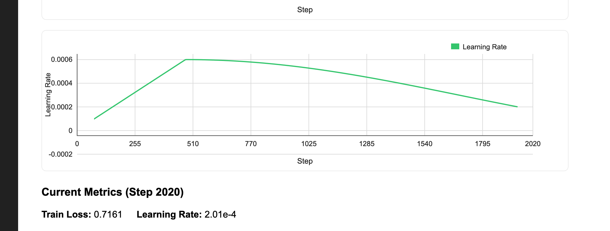
- Cosine learning rate schedule with warmup: We start with a low learning rate, ramp up linearly during warmup (helps stabilize early training when gradients are noisy), then decay following a cosine curve. This schedule outperforms constant or step decay for transformer training.
Checkpointing for fault tolerance
Training a 30B-parameter model for 15,000 steps can take days. Hardware failures and spot instance preemptions are inevitable, which makes checkpointing essential.
class S3CheckpointCallback(L.Callback):
    """
    Periodically upload checkpoints to S3 for durability and resumption.

    This ensures checkpoints are safely stored in remote storage even if
    the training job is interrupted or the instance fails.
    """

    def __init__(self, checkpoint_dir: Path, upload_every_n_steps: int):
        super().__init__()
        self.checkpoint_dir = checkpoint_dir
        self.upload_every_n_steps = upload_every_n_steps
        self.last_uploaded_step = -1

    def on_train_batch_end(self, trainer, pl_module, outputs, batch, batch_idx):
        """Upload checkpoint to S3 every N steps."""
        if trainer.global_rank != 0:
            return  # Only upload from rank 0

        current_step = trainer.global_step

        # Upload every N steps (aligns with ModelCheckpoint's every_n_train_steps)
        if (
            current_step % self.upload_every_n_steps == 0
            and current_step > self.last_uploaded_step
            and current_step > 0
        ):
            try:
                # Find the most recent checkpoint file
                checkpoint_files = list(self.checkpoint_dir.glob("*.ckpt"))
                if not checkpoint_files:
                    print("No checkpoint files found to upload")
                    return

                # Get the latest checkpoint (by modification time)
                latest_checkpoint = max(
                    checkpoint_files, key=lambda p: p.stat().st_mtime
                )

                # Upload the checkpoint file directly to S3 using File.from_local_sync
                checkpoint_file = File.from_local_sync(str(latest_checkpoint))
                print(f"Checkpoint uploaded to S3 at: {checkpoint_file.path}")

                self.last_uploaded_step = current_step
            except Exception as e:
                print(f"Warning: Failed to upload checkpoint to S3: {e}")
This callback runs every N training steps and uploads the checkpoint to durable storage. The key line is File.from_local_sync() which is a Flyte abstraction for uploading files. There are no blob store credentials to manage and no bucket paths to hardcode. Flyte automatically uses the storage backend configured for your cluster.
The callback only runs on rank 0. In distributed training, all 8 GPUs have identical model states (that’s the point of data parallelism). Having all of them upload the same checkpoint would be wasteful and could cause race conditions.
When you restart a failed run, pass the checkpoint via resume_checkpoint so training resumes exactly where it left off, including the same step count, optimizer state, and learning rate schedule position.
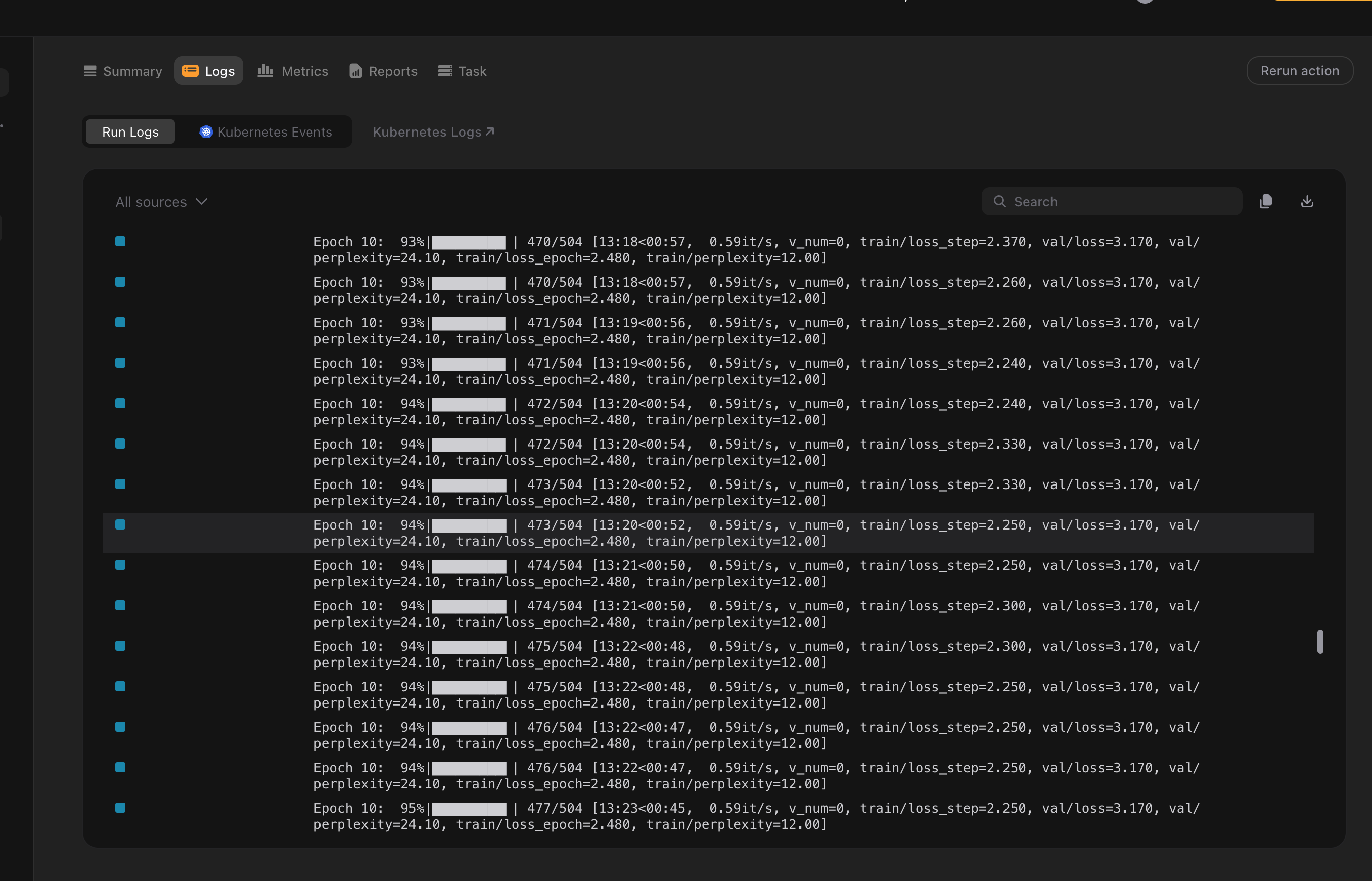
Real-time metrics with Flyte Reports
Multi-day training runs need observability. Is the loss decreasing? Did training diverge? Is the learning rate schedule behaving correctly? Flyte Reports let you build live dashboards directly in the UI:
class FlyteReportingCallback(L.Callback):
    """Custom Lightning callback to report training metrics to Flyte Report."""

    def __init__(self, report_every_n_steps: int = 100):
        super().__init__()
        self.report_every_n_steps = report_every_n_steps
        self.metrics_history = {
            "step": [],
            "train_loss": [],
            "learning_rate": [],
            "val_loss": [],
            "val_perplexity": [],
        }
        self.initialized_report = False
        self.last_logged_step = -1

    def on_train_start(self, trainer, pl_module):
        """Initialize the live dashboard on training start."""
        if trainer.global_rank == 0 and not self.initialized_report:
            self._initialize_report()
            self.initialized_report = True
The _initialize_report method (see complete code) creates an HTML/JavaScript dashboard with interactive charts. The callback then calls flyte.report.log() every N steps to push new metrics. The charts update in real-time so you can watch your loss curve descend while training runs.
There is no need to deploy Grafana, configure Prometheus, or keep a TensorBoard server running. Using flyte.report.log() is sufficient to get live training metrics directly in the Flyte UI.
Streaming data at scale
Training datasets are massive. SlimPajama contains 627 billion tokens and spans hundreds of gigabytes even when compressed. Downloading the entire dataset to each training node before starting would take hours and waste storage.
Instead, we convert the data to MDS (MosaicML Data Shard) format and stream it during training:
@data_loading_env.task
async def load_and_prepare_streaming_dataset(
    dataset_name: str,
    dataset_config: Optional[str],
    max_length: int,
    train_split: str,
    val_split: Optional[str],
    max_train_samples: Optional[int],
    max_val_samples: Optional[int],
    shard_size_mb: int,
) -> Dir:
    """Tokenize dataset and convert to MDS format for streaming."""
    from datasets import load_dataset
    from streaming import MDSWriter
    from transformers import GPT2TokenizerFast

    output_dir = Path("/tmp/streaming_dataset")
    output_dir.mkdir(parents=True, exist_ok=True)

    tokenizer = GPT2TokenizerFast.from_pretrained("gpt2")
    tokenizer.pad_token = tokenizer.eos_token

    # MDS schema: what each sample contains
    columns = {
        "input_ids": "ndarray:int32",
        "labels": "ndarray:int32",
    }
This task does three things:
- Tokenizes the text using GPT-2’s BPE tokenizer
- Concatenates documents into fixed-length sequences (no padding waste)
- Writes shards to storage in a format optimized for streaming
The task returns a Flyte Dir object, which is a reference to the output location. It’s not the data itself, just a pointer. When the training task receives this Dir, it streams shards on-demand rather than downloading everything upfront.
Flyte caches this task automatically. Run the pipeline twice with the same dataset config, and Flyte skips tokenization entirely on the second run. Change the dataset or sequence length, and it re-runs.
Distributed training with FSDP
Now we get to the core: actually training the model across multiple GPUs. FSDP is what makes this possible for large models.
@distributed_llm_training_env.task(report=True)
def train_distributed_llm(
    prepared_dataset: Dir,
    resume_checkpoint: Optional[Dir],
    vocab_size: int,
    n_positions: int,
    n_embd: int,
    n_layer: int,
    n_head: int,
    batch_size: int,
    num_workers: int,
    max_steps: int,
    learning_rate: float,
    weight_decay: float,
    warmup_steps: int,
    use_fsdp: bool,
    checkpoint_upload_steps: int,
    checkpoint_every_n_steps: int,
    report_every_n_steps: int,
    val_check_interval: int,
    grad_accumulation_steps: int = 1,
) -> Optional[Dir]:
    # ... setup code ...
Notice report=True on the task decorator. It enables Flyte Reports for this specific task.
The training task receives the prepared dataset as a Dir and streams data directly from storage:
    # StreamingDataset streams shards from the remote Flyte storage on-demand
    # It automatically detects torch.distributed context
    # and shards data across GPUs - each rank gets different data automatically
    train_dataset = StreamingDataset(
        remote=f"{remote_path}/train",  # Remote MDS shard location
        local=str(local_cache / "train"),  # Local cache for downloaded shards
        shuffle=True,  # Shuffle samples
        shuffle_algo="naive",  # Shuffling algorithm
        batch_size=batch_size,  # Used for shuffle buffer sizing
    )

    # Create validation StreamingDataset if it exists
    val_dataset = None
    try:
        val_dataset = StreamingDataset(
            remote=f"{remote_path}/validation",
            local=str(local_cache / "validation"),
            shuffle=False,  # No shuffling for validation
            batch_size=batch_size,
        )
        print(
            f"Validation dataset initialized with streaming from: {remote_path}/validation"
        )
    except Exception as e:
        print(f"No validation dataset found: {e}")

    # Create data loaders
    # StreamingDataset handles distributed sampling internally by detecting
    # torch.distributed.get_rank() and torch.distributed.get_world_size()
    train_loader = DataLoader(
        train_dataset,
        batch_size=batch_size,
        num_workers=num_workers,
        pin_memory=True,
        persistent_workers=True,
        drop_last=True,  # Drop incomplete batches for distributed training
        collate_fn=mds_collate_fn,  # Handle read-only arrays
    )

    # Create validation loader if validation dataset exists
    val_loader = None
    if val_dataset is not None:
        val_loader = DataLoader(
            val_dataset,
            batch_size=batch_size,
            num_workers=num_workers,
            pin_memory=True,
            persistent_workers=True,
            drop_last=False,
            collate_fn=mds_collate_fn,
        )
prepared_dataset.path provides the remote storage path for the dataset. MosaicML’s StreamingDataset automatically shards data across GPUs so that each rank sees different samples, without requiring a manual distributed sampler. The credentials are already in the environment because Flyte set them up.
FSDP is where the memory magic happens. Instead of each GPU holding a full copy of the model (like Distributed Data Parallel (DDP)), FSDP shards the parameters, gradients, and optimizer states across all GPUs. Each GPU only holds 1/8th of the model. When a layer needs to run, FSDP all-gathers the full parameters, runs the computation, then discards them.
    # Configure distributed strategy
    if use_fsdp:
        from torch.distributed.fsdp.wrap import ModuleWrapPolicy

        strategy = FSDPStrategy(
            auto_wrap_policy=ModuleWrapPolicy([GPTBlock]),
            activation_checkpointing_policy=None,
            cpu_offload=False,  # H200 has 141GB - no CPU offload needed
            state_dict_type="full",
            sharding_strategy="FULL_SHARD",
            process_group_backend="nccl",
        )
    else:
        from lightning.pytorch.strategies import DDPStrategy

        strategy = DDPStrategy(process_group_backend="nccl")
We wrap at the GPTBlock level because each transformer block becomes an FSDP unit. This balances communication overhead (more units = more all-gathers) against memory savings (smaller units = more granular sharding).
One subtle detail: gradient clipping. With FSDP, gradients are sharded across ranks, so computing a global gradient norm would require an expensive all-reduce operation. Instead of norm-based clipping, we use value-based gradient clipping, which clamps each individual gradient element to a fixed range. This can be done independently on each rank with no coordination overhead and is commonly used for large-scale FSDP training.
    # Initialize trainer
    trainer = L.Trainer(
        strategy=strategy,
        accelerator="gpu",
        devices=DEVICES_PER_NODE,
        num_nodes=NUM_NODES,
        # Training configuration
        max_steps=max_steps,
        precision="bf16-mixed",  # BFloat16 for better numerical stability
        # Optimization
        gradient_clip_val=1.0,
        gradient_clip_algorithm=(
            "value" if use_fsdp else "norm"
        ),  # FSDP requires 'value', DDP can use 'norm'
        accumulate_grad_batches=grad_accumulation_steps,
        # Logging and checkpointing
        callbacks=callbacks,
        log_every_n_steps=report_every_n_steps,
        val_check_interval=val_check_interval,
        # Performance
        benchmark=True,
        deterministic=False,
        # Enable gradient checkpointing for memory efficiency
        enable_checkpointing=True,
        use_distributed_sampler=False,  # StreamingDataset handles distributed sampling
    )

    # Train the model (resume from checkpoint if provided)
    trainer.fit(model, train_loader, val_loader, ckpt_path=ckpt_path)

    # Print final results
    if trainer.global_rank == 0:
        if val_loader is not None:
            print(
                f"Final validation loss: {trainer.callback_metrics.get('val/loss', 0.0):.4f}"
            )
            print(
                f"Final validation perplexity: {trainer.callback_metrics.get('val/perplexity', 0.0):.4f}"
            )
        print(f"Checkpoints saved to: {checkpoint_dir}")

        return Dir.from_local_sync(output_dir)

    return None
The trainer configuration brings together all the pieces we’ve discussed:
precision="bf16-mixed": BFloat16 mixed precision training. BF16 has the same dynamic range as FP32 (unlike FP16), so you don’t need loss scaling. This is the standard choice for modern GPU training.gradient_clip_val=1.0: Clips gradients to prevent exploding gradients during training. Combined with value-based clipping for FSDP compatibility.accumulate_grad_batches: Accumulates gradients over multiple forward passes before updating weights. This lets us hit a larger effective batch size than what fits in GPU memory.val_check_interval: How often to run validation. For long training runs, you don’t want to validate every epoch — that would be too infrequent. Instead, validate everyNtraining steps.use_distributed_sampler=False: We disable Lightning’s built-in distributed sampler becauseStreamingDatasethandles data sharding internally. Using both would cause conflicts.benchmark=True: Enables cuDNN autotuning. PyTorch will benchmark different convolution algorithms on the first batch and pick the fastest one for your specific input sizes.
The trainer then calls fit() with the model, data loaders, and optionally a checkpoint path to resume from.
Tying it together
The pipeline task orchestrates everything:
@driver_env.task
async def distributed_llm_pipeline(
    model_size: str,
    dataset_name: str = "Salesforce/wikitext",
    dataset_config: str = "wikitext-103-raw-v1",
    max_length: int = 2048,
    max_train_samples: Optional[int] = 10000,
    max_val_samples: Optional[int] = 1000,
    max_steps: int = 100000,
    resume_checkpoint: Optional[Dir] = None,
    checkpoint_upload_steps: int = 1000,
    # Optional overrides (if None, uses model preset defaults)
    batch_size: Optional[int] = None,
    learning_rate: Optional[float] = None,
    use_fsdp: bool = True,
) -> Optional[Dir]:
    # Get model configuration
    model_config = get_model_config(model_size)

    # Use preset values if not overridden
    actual_batch_size = (
        batch_size if batch_size is not None else model_config["batch_size"]
    )
    actual_learning_rate = (
        learning_rate if learning_rate is not None else model_config["learning_rate"]
    )

    # Step 1: Load and prepare streaming dataset
    prepared_dataset = await load_and_prepare_streaming_dataset(
        dataset_name=dataset_name,
        dataset_config=dataset_config,
        max_length=max_length,
        train_split="train",
        val_split="validation",
        max_train_samples=max_train_samples,
        max_val_samples=max_val_samples,
        shard_size_mb=64,  # 64MB shards
    )

    # Step 2: Run distributed training
    if resume_checkpoint is not None:
        print("\nStep 2: Resuming distributed training from checkpoint...")
    else:
        print("\nStep 2: Starting distributed training from scratch...")

    target_global_batch = 256
    world_size = NUM_NODES * DEVICES_PER_NODE
    effective_per_step = world_size * actual_batch_size
    grad_accumulation_steps = max(
        1, math.ceil(target_global_batch / max(1, effective_per_step))
    )

    checkpoint_dir = train_distributed_llm(
        prepared_dataset=prepared_dataset,
        resume_checkpoint=resume_checkpoint,
        vocab_size=VOCAB_SIZE,
        n_positions=N_POSITIONS,
        n_embd=model_config["n_embd"],
        n_layer=model_config["n_layer"],
        n_head=model_config["n_head"],
        batch_size=actual_batch_size,
        num_workers=8,
        max_steps=max_steps,
        learning_rate=actual_learning_rate,
        weight_decay=0.1,
        warmup_steps=500,
        use_fsdp=use_fsdp,
        checkpoint_upload_steps=checkpoint_upload_steps,
        checkpoint_every_n_steps=model_config["checkpoint_every_n_steps"],
        report_every_n_steps=model_config["report_every_n_steps"],
        val_check_interval=model_config["val_check_interval"],
        grad_accumulation_steps=grad_accumulation_steps,
    )

    return checkpoint_dir
The flow is straightforward: load the configuration, prepare the data, and run training. Flyte automatically manages the execution graph so data preparation runs first and training waits until it completes. If data preparation is cached from a previous run, training starts immediately.
The gradient accumulation calculation is worth noting. We want a global batch size of 256 (this affects training dynamics), but each GPU can only fit a small batch. With 8 GPUs and batch size 1 each, we need 32 accumulation steps to hit 256.
Running the pipeline
With everything defined, running is simple:
if __name__ == "__main__":
    flyte.init_from_config()

    run = flyte.run(
        distributed_llm_pipeline,
        model_size="30B",
        dataset_name="cerebras/SlimPajama-627B",
        dataset_config=None,
        max_length=2048,
        max_train_samples=5_000_000,
        max_val_samples=50_000,
        max_steps=15_000,
        use_fsdp=True,
        checkpoint_upload_steps=1000,
    )

    print(f"Run URL: {run.url}")
This configuration is designed for testing and demonstration. Notice max_train_samples=5_000_000 — that’s 5 million samples from a dataset with 627 billion tokens. A tiny fraction, enough to verify everything works without burning through compute.
For a real pretraining run, you would remove this limit by setting max_train_samples=None, or increase it significantly. You would also increase max_steps to match your compute budget, likely scale to multiple nodes by setting NUM_NODES=4 or higher, and allocate more resources. The rest of the pipeline remains unchanged.
flyte create config --endpoint <FLYTE_OR_UNION_ENDPOINT> --project <PROJECT_NAME> --domain <DOMAIN_NAME> --builder remote
uv run train.py
When you run this, Flyte:
- Builds the container (cached after first run)
- Schedules data prep on CPU nodes
- Waits for data prep (or skips if cached)
- Provisions H200 nodes and launches distributed training
- Streams logs and metrics to the UI in real-time
Open the Flyte UI to observe the workflow execution. The data preparation task completes first, followed by the training task spinning up. As training begins, the Flyte Reports dashboard starts plotting loss curves. If anything goes wrong, the logs are immediately available in the UI.
If training fails due to an out-of-memory error, a GPU driver error, or a hardware issue, check the logs, fix the problem, and restart the run with resume_checkpoint pointing to the most recent checkpoint. Training resumes from where it left off. Flyte tracks the full execution history, so it is easy to see exactly what happened.
Going further
If you’ve run through this tutorial, here’s where to go next depending on what you’re trying to do:
You want to train on your own data. The data prep task accepts any HuggingFace dataset with a text column. If your data isn’t on HuggingFace, you can modify load_and_prepare_streaming_dataset to read from S3, local files, or any other source. The key is getting your data into MDS format. Once it’s there, the streaming and sharding just works. For production training, look at SlimPajama,
RedPajama, or
The Pile as starting points.
You want to scale to more GPUs. Bump NUM_NODES and Flyte handles the rest. The main thing to watch is the effective batch size. As you add more GPUs, you may want to reduce gradient accumulation steps to keep the same global batch size, or increase them if you want to experiment with larger batches.
Your training keeps failing. Add retries=3 to your task decorator for automatic retry on transient failures. This handles spot instance preemption, temporary network issues, and the occasional GPU that decides to stop working. Combined with checkpointing, you get fault-tolerant training that can survive most infrastructure hiccups. For persistent failures, the Flyte UI logs are your friend as they capture stdout/stderr from all ranks.
You want better visibility into what’s happening. We’re actively working on surfacing GPU driver logs (xid/sxid errors), memory utilization breakdowns, and NCCL communication metrics directly in the Flyte UI. If you’re hitting issues that the current logs don’t explain, reach out. Your feedback helps us prioritize what observability features to build next!